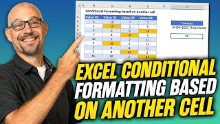
Colour a Row in Excel Based on One Cell's Value

ฝัง
- เผยแพร่เมื่อ 22 ธ.ค. 2010
- In Excel, follow these steps to check the value in one cell, and colour all other cells in that row, if the value is above a specified amount.
Watch this video to see how to colour a row in a table, by using Excel's conditional formatting. A formula checks one cell in each row.
To get the Excel workbook, go to my Contextures website:
www.contextures.com/xlcondform...
Instructor: Debra Dalgleish, Contextures Inc.
Get Debra's weekly Excel tips: www.contextures.com/signup01
More Excel Tips and Tutorials: www.contextures.com/tiptech.html
Subscribe to Contextures TH-cam: th-cam.com/users/contextu...
#ContexturesExcelTips
VIDEO TRANSCRIPT
With Excel's conditional formatting, you can easily highlight a cell if it's over or under a certain value, or if it meets a value that you've set.
But in some cases, instead of just a single cell, you might like to highlight a whole row in a table, if one of the cells in that row is over a certain number or under.
In this case, we would like to highlight each row in this list if the number of units sold is greater than 75.
So to do that, I'm going to select all of the rows, all of the columns in each row. So I've selected from A2 down to D10.
On the Ribbon, on the Home tab, I'll click Conditional Formatting, and none of these preset rules will do exactly what I want. So I'm going down to New Rule, and in here I'll select a formula.
So I'm going to use a formula to determine how to color each row.
When I click that, there's a spot where I can put the formula.
I want to, in each row, look at the value that's in column B. So I'll type =
And we want, from every column, we want to look at column B. So we have to lock that cell. We don't want it to be relative, we want it to be absolute.
So type a $ to lock that in. And then B.
And we want, in this case, the active cell we can see is white, where the other cells are highlighted with blue.
We can see that, in the name box, A2 is showing up. So that's the active cell, so the active row is 2. So I'm going to type 2 here.
We're going to check what's in B2 and see if it's greater than 75. So that's our test.
And if it is greater than 75, we want to format it. So I'll click Format and I'll choose a fill color, maybe a blue color and click OK, and click OK again.
And now, any row where the number of units is greater than 75, all four cells in that row are colored blue. - วิทยาศาสตร์และเทคโนโลยี


This is by far the most helpful explanation I've come across - it makes sense to people who don't ordinarily understand how codes and referencing works.
Thank you!
MANY THANKS!!! By far, THE BEST and Easiest excel tutorial...thanks.
Very Helpful. Saved me a lot of time and learned me exactly what I needed. Thank you!
Such a complicated task in excel, made very simple. Thanks a MILLION!
Short and very useful! Thank you angel!
Thanks. Clearly explained in the vid. Very useful. I used it with word "Completed" and highlighted the entire row in Green.
Short and to the point! Thank you!
You're welcome, Joey, and thanks for your comment!
2019 and still very helpful. Thank you so much
Oh wow..... thank u thank u thank u... been searching fro this everywhere..... could format only 1 cell.... this was really helpful for me to format all the cells at once.....
Thanks, that was so simple and clear
I changed color of cells of one column to green/red based on value(+positive or -negative)
Thanks for this useful tutorial video. I have date that I wanted to apply the formatting conditions on it but I couldn’t. I want to change the whole row based on a dropdown list “letters”. Any tips?
This is exactly what I am looking for. Amazing. Thanks for sharing ❤❤❤
You’re welcome, and thanks for your comment - I appreciate it!
For anyone who wants this to work with a particular word, substitute the >75 in the example with:
="yourword"
This is very helpful. Thank you !!
Loved the way it was explained slow an easy.
Thank you for this!
I love this! Straight to the point...exactly what I need but there is just 1 issue with this. It won't let me highlight everything in the area I selected due to a merged cell. It only highlights the top row...not the whole thing. How can I get around that? I would also like to know how I can highlight a word every time it is typed. How can I do that? Thank you.
You are bloody awesome!!!! Thank you!
i loved your video, thanks!!!
Very useful, thank you.
Perfect, thank you.
Thanks very much indeed for this - short and to the point. Very pleasant voice too.:-)
Just what I needed. Thanks!
You're welcome, Adam! Thanks for letting me know that it helped you!
Crystal clear. Thank you.
Thank you, Nicole!
Amazing, thank you! 👏🏻 perfect tutorial and have achieved what I needed with a little tweak. I chose to use ="published" as I didn't want a value.
You're welcome, Amberley, and thanks for your comment! I'm glad you were able to add that tweak, to get exactly what you needed
Helpful, thx!
Awesome. This is so simple and so useful
Thank you, Latha!
Very helpful. Thank you.
You're welcome! Thanks for letting me know that the video was helpful to you
super helpful
Thank you very much.
Amazing Tutorial on excel thanks :D
Thanks!
Thank you!!!
Excellent explanation!
Thank you, Audie!
Thanks!
How can similar be used for formatting columns?
Thanks so much
Thank you.
thanks Matthew! Just a side note,retain the "". example, =$J6="Received"
Bingo! Thanks!
Two questions:
1. How do I go about applying this condition to a blank excel sheet to be used among several users later? Where do I highlight before creating the rule? I'm not able to select (A2-D10) as I'd like for the rule to apply to the entire page as long as data inputted matches.
2. How do I limit the color fill to cells with data only, and not the entirety of the row(s)?
THANKS MADAM
How can this work with text? Say column G has various words used, like 'Pending' and Cancelled' With the cells in column G already set with a 'Conditional Formatting' rule to change the cell to a specific color. I want the row to change to that specific color. Can this be achieved with this similar process?
THANK YOU!!!!!!!!!!!!!!!!!!!!!!!!!!!!!!!!!!!!!!!!!!!!!!!!!
You're welcome, Viktoria, and thanks for your comment!
THANK YOU THANK YOU THANK YOU
You're welcome! Thanks for watching the video
How do you do exactly that except using a formula for numbers between rather than above or below a certain value
Thanks for the video. I have a question. So the formula is =$B2>75. Basically the idea here is to compare each cell in column B with 75 if true the color the row corresponding to that cell to different color. Since i am going to compare all cells in row B then why I need to fix B. It is already fixed if I comparing each cell in column B. I am moving like this B1,B2, B3, B4, B5 etc. So why I need to fix B. also what tells excel to color that row? the formula is just to compare but where is the part that tells excel to format the row when the condition is true. I am just trying to understand the logic but it is not easy. Thanks a lot once again
This is just fantastic! I needed to know this, but while I can have the entire row highlighted, I'm having trouble with something similar. I want to highlight an entire range with multiple rows, but it only highlights the first row. I think that $ lock helps to get the first row, but it doesn't do the rest, which I think are becoming relative to the row of the formula target. I wish I could just tell it "hey Excel, highlight this whole range if this one cell has this value/text...." Any help is greatly appreciated. Thanks
+Jason Cramer Actually I figured it out. if the cell in my formula in question is A1, I had been using $A1, but what's required in order to use this on a whole range I need $A$1. Just fyi for anyone who might want that answer.
Very concise. Instead of UNITS, I have changed it to GENDER. Can anyone out there help please ?I'm from Singapore.
...but I have multiple sets of rows with same values in my sheet and I want to color the sets that have values of say, 82 - blue, 83 - green etc...they also go down with decimals and I'd love to automatically color them rows with lighter shades...sorry for ruining your day but I'd really like to know how can I do that :-(
I wanted to find all yellow filled cell in B column and put a "OK" or checkmark in A column! how is that possible? thanks
You could filter column B based on the colour, and then enter the OK in column A for the visible rows.
How to with strings?
how can i do this with a column not a row?
פשוט וטוב...
How to do formatting for equal to value.
Hello
How to highlight the row in case we want the cell to highlight equals to a certain text value. In that case what formula would be applicable in conditional formatting. Please help.
=$B2 = DummyText This gives me an error.
Thanks!
I am 2 years too late, but the reasoning is because you need quotes, ran into the same issue myself.
=$B2="Dummy Text"
dear please tell me....if one cell is in color then other cell automatic colored???????
No, Excel's conditional formatting only works with values, not cell colour
👍👍👍
Thank you!
Right now my computer speakers are hooked up to my TV. I got a new TV and wanted to try the upgraded Bose speakers from my computer to see if they work, and they do. Anyway, I can't listen to the video "Color a row in Excel based on one cell's value". I am very advanced/proficient in Microsoft Excel. so I was hoping you could just tell me the steps real quick? Again, I know what I'm doing and I'm familiar with conditional formatting, so it should be easy to tell me because you don't have to start at square one like I'm a beginner. If you're not up for it, I understand. I can probably guess, but it's almost quitting time and I thought you might know off hand. I have Excel 2007, if that makes a difference. Either way, thanks for your website it is pretty cool. If you ever need any help I know how to use all the formulas you mention in the other videos and I'm not just saying this I am quite advanced. I've had Vlookups that link to a match formula and math formulas that are 2 paragraphs long (I worked as a Software Engineer at NASA Goddard Space Flight Center for 12 years). I know pretty much all those formulas (including the Engineering add-ons like hex2dec), the stat formulas like countif, etc.. like the back of my hand.
I can send you some of my work if you are interested. In fact I created, completely in Excel with some VBA) a NASA standard cost report that links from our original estimate (that I also made in a separate Excel file) to the actual costs (another file downloaded from Microsoft Access) to see how actual/plan costs compare, and then the future costs are projected out three months. I made it all in Excel and the company I worked for (the NASA contractor) used my system for the next 5-6 years. And these formulas linked across different worksheets and workbooks.
I promise I'm not trying to brag, I'm just excited to see a website about Microsoft Excel. I never felt like all that stuff I learned just doesn't have too much of a market, but I love making spreadsheets and I can make them so easily, probably just like you.
If you can help with that conditional formatting question, I would appreciate it. Otherwise, have a great day.
My name is Celeste, and I'm from Annapolis, Maryland. Thanks!
Just a reminder: don't include the fist row
bad vidio