Excel - Use Conditional Formatting on a Cell Based on Another Cell's Value

ฝัง
- เผยแพร่เมื่อ 28 ส.ค. 2024
- full blog post: odyscope.com/ge...
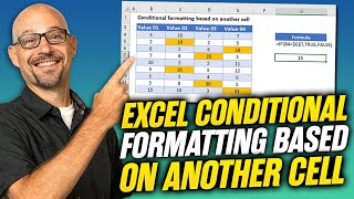
Problem: You want to use conditional formatting on a cell or range, based on another cell's value.
Solution: Create a new conditional formatting rule and select the option to "Use a formula to determine which cells to format".


Thank you! You're the first person to explain this in a clear, straight-to-the-point way!
An outstanding tutorial! Far too often I find that contributors here on You Tube leave out small parts of a particular process, leaving users frustrated and aggravated.
Everything here was clear, concise and to the point. I was able to learn this process without even having to watch the video a second time. Well done!
This is a brilliant tutorial. Short, simple and straight to the point. Instructions were excellent pitched exactly at the right level for a non proficient excel user. Thank you Chris
Relevant and useful 9 years later! Quick and easy to follow…thank you
Good job Chris! You took something and broke it down in a systematic, concise, and discernable manner. It is one thing to teach someone, but it is all together a higher level when you are able to achieve this with brevity! Well done.
Thanks for the clear explanation. Watched a dozen of these and yours was the first I came across that took the time to point out the Dollar sign needs to be removed from before the row number.
Precisely what I was looking for. Thanks for making it concise!
Thank you for teaching example in a precise and clear way instead of adding unnecessary words
Excellent tutorial. I had to adapt it to Excel for Mac, but because of your excellent communication style I was able to find the differences quickly.
How can you use the ''equal to'' preset conditional formatting in excel to format multiple values in a range at once and not one at a time? Or if there is a better alternative to this conditional formatting, what is it please?
Awesome, thanks. I wanted to do this and was searching online; the steps in the tutorials were not clear until I stumbled on this one... Thanks a lot; Keep up the good work
Thank you. Something so simple that I couldn’t find the answer to until I found your video.
You can't imagine how much your video was helpful ,i saved a lot of time , thank you so much.
Thank you! After 8 other videos I finally got my answer, appreciate the quick tutorial
Under 5minute video and straight to the point keep it up👍
Thanks. I subscribed just because you were very straightforward and you explained it well.
Thanks, I would have thought this would be more self explanatory but you did a great job!
Thanks for the help, I've been wasting hours formatting hundreds of cells (didn't know about the '$' formatting).
Thanks for this. Took a while to find a solution, but you have now solved it for me. Cheers!
Wow that was a great video. I was getting so frustrated trying to figure that out and this video just made it so easy. thank you!!
thanks. i saw a few videos but no one mentioned how to copy formatting with reference to a respective cell. it was always referring to a common single cell.
so simple yet so helpful, keep up the good work! saved me so much headache and frustration, so glad i found this!
4 hours to find this GREAT video!
Thank you, GEEZUS I was struggling.
Exactly what I was looking for! Thanks!
Thank you for the video, it helped me to finish a template report that needed to insert some conditional formating using formulas.!!
Thank you so much!!!! you just saved me from an exam!
Thank you for sharing. Short and sweet
Awesome... clear, concise, just what I was looking for.
It was the last step I could figure out on my own.
Thanks!
That was so helpful..thanks man, I have been looking for that solution for so long
Exactly what I was looking for. Thank you.
Hi Chris. Thanks for your info. Can you tell me how I can ignore a zero (0)? I have a format that highlights blanks but 0 is not blank.
Tks.
Thanks! The fundamentals here allowed me to expand and go another direction! Appreciate your knowledge!
ATB,
David
Just the format rule I was looking for.Thanks
I'm struggling to find the answer to this so hopefully you are still active. I want to conditional format based on a cell but that cell is a calculated value (example =e3+1). Is this possible? I can conditional format if there is no formula but as soon as I go to format based on a calculated cell it refuses.
Great! I spent a few hours yesterday trying to figure out how to do this!
Thank you so much for releasing such a great work and that is exactly what i'm dying to look for to solve my homework. And beside learning excel tips, i get to practice listening skill as well.
Thanks! Very clear explanation!!!
Great video, it helped me a lot. I am trying to format another cell range when looking for a specific word and I can't find how to do it
Thank you! Really helpful for formatting a spreadsheet I'm using for students' results during the lockdown!
Excellent tutorial! Concise and well-explained.
Thanks so much for sharing. I was looking to do so for a while now...
Exactly what i was looking for. 👍👍👍👍
Excellent tutorial, thank you
Hello Chris,
I am great fan of yours and learned lot of excel formulas by seeing your vedios.
Now i need a help hope you would help me in our office we have a daily tracker in that we have 12 agents and works in 24/7 shifts we work on incident tickets as soon as the ticket arrives we have enter the ticket number in that sheet and change the color of the cell manually according to the time the ticket arrived for eg. if ticket came in between 8am to 9 am it will be green if it is between 9 am to 10 am then red if it is between 10 am to 11 am then purple so on so instead of changing the color manually i need a formula or a steps so based on current time when the data entered into a cell the color should change please suggest
Great video and explanation Sumit
Great and detailed insturction!
You are simply awesome sir ❤️
Still works!! Awesome vid
Thank you for the tip. I appreciate your taking the time.
I am stuck with a case where I need to compare two cells and change formatting based on the value in the other cell, I don't have a fixed number like greater than 60 or less than 60. For each cell the value will compare with the value in the other cell and of it is greater or less than that value the formatting should change. Can anyone help or give reference to a video tutorial?
Excellent and simple to understand...Thank you..
How do you format if a cell "contains" text
In the example below I would like Column C to formatted yellow if the word "partly" is in the Column E
E4 Work partly completed - Because of fault
E7 Work partly completed - Because no materials
thanks, you made it clear and easy
Thanks for the great videos, but I have a question. if I have have a cell with a number and I want to make sure that this number highlights if it ever goes above more than 10% of another cell, is it possible to use conditional formatting for this.
Nailed it, exactly what I was looking for, thanks!
Very clear and concise. Thanks
Thanks. Just what I'm looking for.
Thank you. This is great. I have a similar problem like this one with a twist! See if you can come up with a solution, please! I want to make the fill color of a cell in a row based on the comparison of the value of the current cell and the cell to its left. If the current cell value is larger than the value of the cell to the left, then I want to fill it with green, if it is equal, I want it to be filled grey, and if less, I want it to be filler yellow. Is that possible?
Thank you so much! Was perfect for what I was trying to do in my project.
how do you format based on another cells value which is a range for example (=$B$13=Source!$H$127:$H$150) if i am only worried about one value then this works (=$B$13=Source!$H$127) but what if any value on b13 is between H127:H150
Why does line number 4 was impacted by the formula? It supposes just the >60 will highlight?
Thanks ... Really
I have found the exact solution I am looking for.
what if you want to do it actually based on another cells value and not based off a flat value like 60? like $E2 > $B2 --- should it it be comparing to E2 > B3 in the next row and so on?
Hey, tnx for sharing a great video. I've got questions though. How are you gonna modify your formula if you wanna highlight a cell from an array of lookup cells based on the value of another cell, e.g. you have a list of employee IDs in an array and you are using say, Index function, to lookup for an employee's ID, and whatever lookup value you have it will highlight the ID in the lookup array? tnx!
What if you want to see is another cell is lower than the cell you are conditioning?
like =if(c4 < f4) then do something
Hi,, great video.. in Row 4, the days outstanding is 14, yet the rule still applies to this row. How is that ?
Thank you very much.
Exactly what I was looking for.
Thanx a lot, exactly what I needed to know :-) Good job!
Great tutorial, learned exactly what i needed to
How do i use conditional formatting to link the accumulated numbers of individuals into totals
Dang, that helped me so much. Thank you so much, I just subscribed to your channel :)
Thanks, you made my life easier!!!
Nice Video Sir. I have a question Sir, how to use conditional formatting on Month.. when i want only the month of January, April and October? can u teach me the formula? thanks
Such a big help Thanks
you rock, spinning my wheels on this today!
Thanx! I've been wondering about this trick for years. I guess my mistake was in understanding what the cond.formatting formula is supposed to be.
Can you use the format painter to copy the formatting down a column, if you use a formula to determine the format?
Hi Chris,Have a question. So in one cell (A1) I have a number which can vary and in another cell I want to use a formula that can also vary depending on the number in A1 and the result of that 2nd number multiplied by a dollar amount reflected in another cell. Example B2 is a percentage of A1 and if A1 is 100 to 200 I want B2 to be 15% of A1, then in C2 that % number from B2 x $100. So if A1 is 100 then B2 would be 15 and C2 would be $1500. First part I'm stuck at is the range 100 to 200 in A1.Here's where it gets even trickier. If A1 is 201 to 300, then the same formula with a lower percentage. So let's say A1 is 250, then I want 12% of A1 in B2 and that number x $100 in C2. If A1 is 301 to 400 then the % of A1 is 10% x $100. So the % drops with a higher number in A1. Can you provide any help, say a formula?
I wanted to calculate a tons of number with text on it?
I wanted to either delete the text or just ignore and continue to calculate the number?
Will it carry to new rows added if I only select the current rows in the table?
In my case I want to show a red arrow next to the value indicating that the amount has increased or a green arrow indicating that the value has decreased? Any way to create that rule?
Unfortunately this doesn't work. If you pause at 3:09, you will see that the accounts that should be highlighted are not. For example, you can make out that there is an account that is 104 days over due but it is not highlighted while one with 57 days is.
I don't mean to nitpick, it just that I am having the same problem and have yet to find a solution.
Looks like all are shifted up one cell in the first column. The example he shows at 1:02 is correct, the one at the end is one up from that. He did the formula on cell A1 while that is a header, the list starts at A2. I think that's where it went wrong.
How do I change a value in one column, based on another column value? For instance, if my column labeled "Debit or Credit" value is "Credit", I want to change the value on that row in the "Transaction" column to a negative value. Right now all "Amounts are listed as positive whether they are a debit or a credit.
Many thanks
How about indenting text in one cell based on the number in another cell (in the same row?)
A Great video, exactly what I needed!
Is there any way you can make a video showing how to have a drop down menu and once you select 1 value in that menu it will auto fill 2 other cells with information. But in saying that the other 2 cells with be filled with different information.
Can you help? I have the DATE in one cell and I want the DAY to auto-populate in another cell base on the date.
What if I want it to be red if greater than 60, blue if equal to 70 and black if greater than 80?
We need to select 1st cell of the criterion rule to work this out correctly, he selected E2 instead of E1 2:19
if you want to assign a variable to an account number with multiple entry in the worksheet, how do you do that?
That's exactly what I'm looking for! GIG 'EM!
Hey Chris, could you do a video (if this is possible) on how to change on cell's background/color based on the value of a different cell? For example, a column of values are conditionally formatted to show as a 3 color blend of red,yellow,green based on the value, however, you want that color to carry over to a different cell without the value in that different cell being changed. This is possible?
can i apply two of the same formula on one cell? like if it says value "xyz" then it turns the other cell green otherwise red? please help me with this
Some " reds" in colummn A , In "E columm"n in less than < 60 , not > 60 , like you defined "?
Cell A4 is red but E4=14 and not >60 ... Looks like there is a problem with the formula and it is not working as expected.
HOW TO DO CONDITIONAL FORMATING WITH CHECK ICON
WHEN MET THE CONDITION?
Thank you for sharing, have a graded presentation to do and I believe this will help me sooo much
Hello Chris. Could you please help me? I work in the collections dept of a business. We have excel sheets, which cathegorize customers according to the time it has passed since they bought our equipment (0-30; 31-60; 61-90; 91-120 and 121+) I'd like to know how to format each column at the time in order to have the names of the customers highlighted according to the amount they owe us? Thanks for your help Chris!
Hi Luis, you can use the same technique shown in this video, only in your case you will have to put in 5 rules - one for each category. Your first rule should be =cell#>120 and select the formatting of your choice, the second rule will then be =cell#>90 and again you select the formatting you want for customer in the category 91-120; and so on until the fifth rule =cell#>0. Note that Excel applies the rules in the order you enter them, so be sure to enter a rule for the highest bracket first and walk your way back to 0. Hope this helps.